Today we will be looking at how to go about data pre-processing in R. This can be done by reading in some arbitrary data. You can find data sets using this link : https://www.openml.org/
We want to begin by reading the data in from the file, which can be done by using this function:
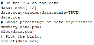
Once the data is read in, it’s possible to do a lot with it. We’ll start with PCA, which essentially reduces dimensionality by combining attributes to form principle components. These principle components then represent a percentage of the data.
To do this in R, we use the following code:
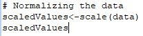
Now we’ll look at scaling the data, which is also known as normalizing the data. This is a process of converting attribute values into new values within given bounds, usually [0,1] or [-1,1]. This can be done in R as follows:
Regularization is intended to solve overfitting problems in machine learning through a loss function with two main types; L1 and L2.
Next time
That’ll cover it for this one, next time we’ll look at visualising data in R.
Today we will be looking at the object orientation concepts available in Python. Python is an object-oriented language and offers much functionality that would be expected to come with such status. You can write classes, instantiate objects and inherit from other classes etc.
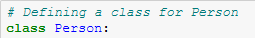
Let’s start by declaring a class, this is done as so:
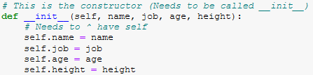
Then we’ll need to write the constructor. In Python, this is a little different to any languages we’ve seen previously:
The “init()” function acts as the constructor, and note how it has been passed “self”. Ths is used to represent an instance of a class, so that the class knows which object it is operating on. This is different to something like Java, where you only need to use the “this” keyword to remove ambiguity from the code.
It is important to bear in mind that most functions you write in Python will require “self” to be an argument.
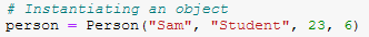
When it comes to actually instantiating an object of the class, interestingly enough, we don’t have to pass “self” to the function. We just declare the object name, assign it the constructor with the required arguments, as seen below:
This means you only have to worry about “self” when it comes to writing the actual classes, and not when you’re using the classes in your code.
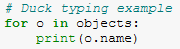
Lastly, we’ll be looking at “duck typing”, which is a type system whereby the type of the object is less important than the method it defines. This means that when the Python code is compiled, instead of checking for types, they check for the method or attribute the object is using.
This means that you can have a list of objects displaying their name attribute, and as long as each type of object in that list has this attribute in its class definition everything will be okay. This is shown below:
Then, if the object doesn’t have the method, an error will occur.
Next time
That’s if for this time, next time we will be looking at mathematical functions, pure functions, anonymous functions and functional operations. In short; a whole lotta functions!
Today we will be looking at loops and control statements in C. By this point, assuming you’ve followed the other tutorials on the blog, you should be very familiar with these structures.
In C, we have access to:
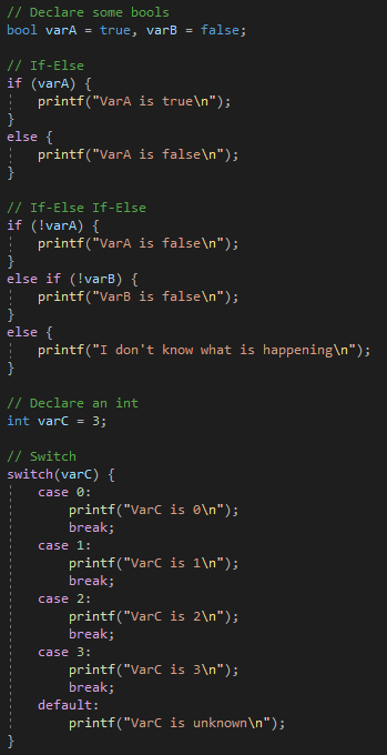
if
else if
else
switch
For our conditional statements. And then for our loops we have access to:
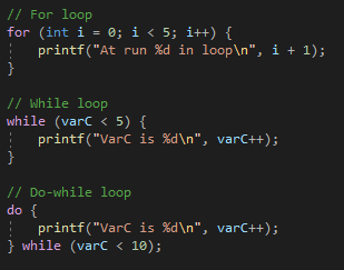
for
while
do while
Examples of these can be found below:
You may notice they look very similar, practically identical even, to the syntax for the loops and conditionals in Java. It’s one of the reasons why people tend to say once you have learned one language, you can easily pick up more.
But C also has another kind of control statement; “goto”. This statement essentially tells the code to jump to a specific point in the code. Whilst this may seem great on paper, it is recommended to avoid goto, as it cam lead to buggy code, or code that is too hard to follow. It can also allow you to jump out of the scope, which can be problematic for variables in the program.
And this concludes the C tutorial series, next we’ll be going through C++. If you haven’t checked out any of the previous tutorial series, I’d highly recommend you do so. Please consider subscribing to either YouTube channel or the blog if you haven’t done so already.
Thank you very much for reading and I’ll catch you in the next one.
Up until this point we’ve been using header files that are provided as standard with C. But what if we wanted to make our own header with functions that we could then include in our other projects. Today we will be looking at this process.
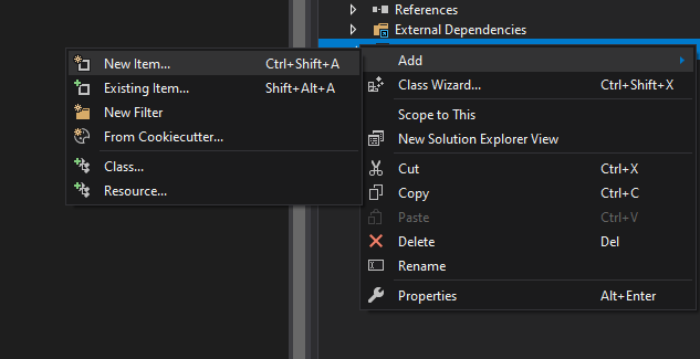
Firstly, we’ll want to create a header file and give it a name. In Visual Studio, we can do this by right clicking in project solution pane and selecting “Add -> New Item”. In the projects we’ve been using, there is a dedicated “Header files” directory that we will add it to.
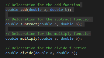
With the header file created we can now declare some functions. We’ll declare the four basic mathematical functions for simplicities sake:
Note how we haven’t written the body of the functions yet. By convention this should be done in the corresponding “.c” file (“.cpp” for this tutorial), so we’ll go ahead and make that next.
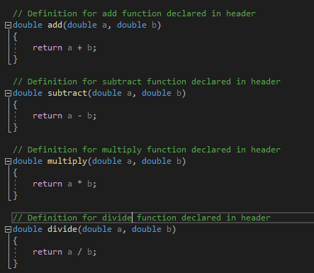
In this new file we now want to write the definitions for all our functions that we placed in the header file.
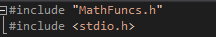
Now that we’ve created the header file and written the function bodies, we’re ready to test using this header file. To do this, we use the “#include” statement as we did previously, only this time, instead of using “<>” to contain the library name, we’re going to use regular speech marks.
This then gives us access to all the functions in the header file, which we can test with the following code:
And that about covers header file creation in C.
Next time
Next time we will be looking at conditional statements and loops, as well as the illegal GOTO statement.
R, much like any language, has the capacity for looping/iterating. This means that we can work over a sequence of objects, performing operations, appending values etc.
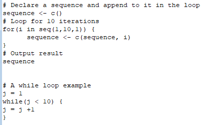
In R, loops can be declared like so:
However, if you try and run this code, it may take some time. This is because loops are not very efficiently implemented in R, and there is a good reason.
R has a function called “apply” which is the preferred way of implementing looping. It can seem a bit weird at first so let’s examine how the function works.
The apply function is used to execute some functions on a matrix or vector. Since R utilizes mostly vectors and matrices, this works out well, hence why the apply is preferred over for loops.
The apply syntax is really simple actually:
apply(<variable>, margin,<function> )
Where variable is your variable (matrix or vector), margin is whether it should be operating on rows or columns (or both), and function is the function you want to use.
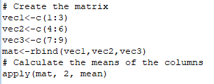
Let’s take a look at it in action:
In addition to apply, there exists several other similar functions for different data structures:
lapply; for performing operations on lists
sapply; for applying a function to each element of a vector, list of dataframe
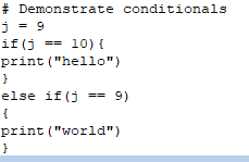
Now we’ll look at conditionals, so that we can make our code do different things. Much like other languages, R has the classic IF/ELSE constructs:
You can see that the syntax of R is really quite similar to that of Python, especially if you’ve been following the Python series on the blog.
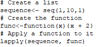
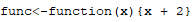
It is also possible to create your own functions in R, which can be useful for generating data points or for plotting mathematical functions. To create a function in R, the following syntax is used:
It is important to remember that R is dependent on the curly braces for defining blocks of code, unlike in Python where the indentation determines the block of the code.
Lastly, we’ll try and apply a function we’ve created to some vector.
And this has completely replaced the loop functionality and executed much quicker.
Next time
Next time we will be looking at reading in data from files, performing PCA and scaling/regularization on data.
Last time we looked at some data types we had available in Python as well as control structures, functions and overall indentation.
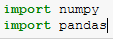
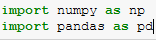
Today we’re going to be looking at NumPy and Pandas. We’ll need to start by importing them which we can do as so.
We can also abbreviate the name at import by doing the following:
This means we can use are shorthand name for the package.
NumPy essentially offers us a robust array schema, with numerous functions available including calculating the mean, standard deviation and even the covariance matrix for a multi-dimensional array.
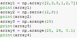
But first we’ll need to declare some NumPy arrays. Some examples of how to do this are shown below:
This then provides us with a robust way of storing our data for manipulation, however, maybe we want something more akin to a table when doing our data analysis.
This is where Pandas come in. Pandas let you create DataFram objects, which are essentially tables of columns and rows, with headers and the data stored within the table.
We can create Pandas like so:
We can access data entries using “iloc” but there are other functions available.
These two objects can be converted from one to the other which makes it incredibly easy to do machine learning and data analytics.
That’ll cover it for this time!
Next time
Next time, we’ll be creating classes, instantiating those objects in our applications and duck typing!
Last time we examined the variable types available to us and discussed how there were many possibilities for things we could do with arrays.
This time we’ll be putting some of these ideas and concepts into action by writing functions and demonstrating recursion.
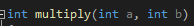
Declaring a function in C is done like so:
It is very similar to Java that we’ve seen before. You have your modifier, your return type and your function name, with any arguments being included in the brackets.
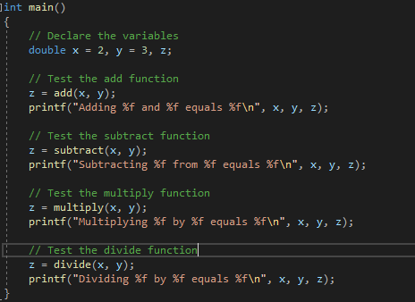
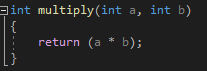
With the function declared and with it taking some arguments, we’ll have to write the body. We’ll write a function that takes three numbers and multiplies them together.
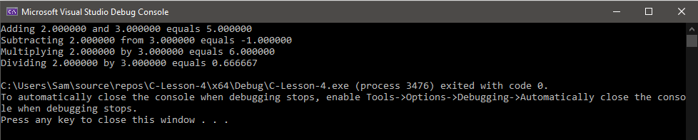
Now when we call that function, we’ll pass it three values. Those values will then get multiplied together and the result will be returned.
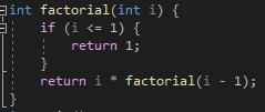
We’re now ready to write something recursive, which simply means that the function calls itself whilst executing. Those executing functions will then call themselves and so on. This is a more resource heavy way of programming, but since resources tend to be cheap nowadays, recursion is a really neat way of writing code.
Here you can see that factorial will keep calling itself with an update value in the return statement unless a condition is met. If there condition were not there, the application would run indefinitely, with the number of functions being called growing exponentially.
So that will cover functions for this tutorial!
Next time
Next time, we will be looking at header files in C, how to make them and use them in our projects and the benefits they have.
So last time we did “Hello World!”, a classic start in programming and the introduction I had when I started teaching myself C.
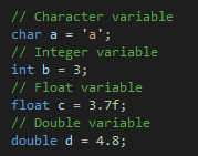
This time we’re going to be looking at the variable types available in C. In C we have access to four main variable types:
char
int
float
double
We’ve seen these before in the Java series, so if you’re unfamiliar with what these variables are, feel free to check the Java series out on the blog.
We’ll take a look at declaring some variables now:
As you can see the syntax is very similar to the other languages we’ve looked at thus far, so if you’ve been following along there you’ll have no problem taking to C.
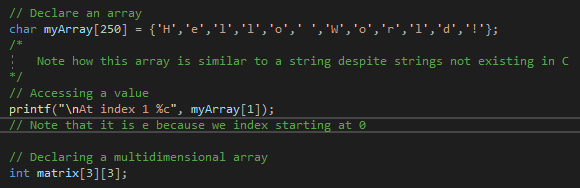
It may seem like we cannot do a great deal with C since there are so few variable types, but C does support arrays, which opens up more possibilities.
Arrays can be declared like so:
Remember to specify the size of the array, and ensure it is big enough to encompass the volumne of information you’re working with.
C also supports the creation of multi-dimensional arrays.
The inclusion of arrays allows you to do much more with your application, since char arrays can act as strings and you can store data with multiple dimensions.
Next we’ll be looking at comments, so that you can add notes to your code.
There are two types of comment in C and we’ve seen them both before in Java.
“//” For a single-line comment
“/**/” For a multi-line comment
C and C++ are very similar, but C++ supports object-oriented programming. This is because C++ was developed as an object-oriented extension o fthe C language. The C language is by default built into the C++ language, which means that you can regard C++, for all intensive purposes, a superset of C.
There is plenty of information that highlights more of the differences between the languages, such as the C++ has a greater emphasis on type checking. But for now we’ll assume that C++ just builds on C.
Next time
Next time, we’ll be looking at declaring and writing functions, as well as making a recursive function.
Last time we got all set up in R and now we’re ready to start writing some scripts.
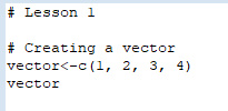
Firstly, we’re gonna look at vectors. These are sequences of data elements that consist of the same basic type.
We can declare them like so:
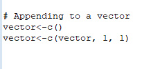
And then we can even append to them too:
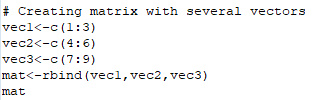
These are then useful for if we want to combine several vectors into matrices like so:
Matrices in R is essentially a two dimensional array with atomic types in it.
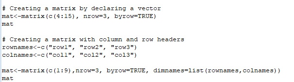
There are several ways of creating matrices, shown below:
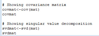
With these data types you can do many different functions relating to matrix mathematics, and even machine learning because of the nature of the data structure.
Some examples of what can be done with matrices and vectors are shown below:
Next time
Next time, we will be looking at looping in R, conditionals and other functions that we can use.
Today we’ll be looking at data types in Python. Python is an object-oriented language and doesn’t actually require a type declaration when creating variables. Nevertheless, variables will come under a few categories.
Numeric
Boolean
Sequence
Dictionary
Numerics include integers, floats and complex numbers:
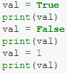
Booleans are true or false, as we’ve seen in other languages:
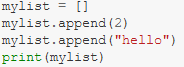
Sequences include strings, lists and tuples:
And a dictionary is an unordered collection of data in a format:
When coding in Python, you may have noticed that there are no curly braces, this is because the compiler is looking at your indentation to define blocks of code. Using tabs will cause an indentation which can be used to define blocks and sub-blocks of code.
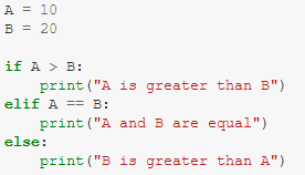
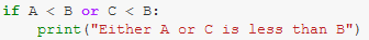
Now we’ll look at conditionals and loops. Conditionals in Python are a bit different to other languages, you have IF, ELSE and ELIF (which is the equivalent of ELSE IF):
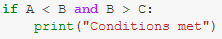
Python also implements logical AND and OR by using keywords:
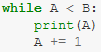
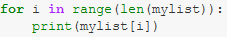
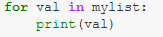
There are several types of loops available in Python, those being:
While loop
For in loop
Index iteration loop
The last thing we’ll be taking a look at is functions in Python. These can be declared using “def”:
This function takes two arguments and adds them together. Note how in the functions, loops and conditionals we’ve looked at, there is a colon after before the indentation begins.
Next time
Next time we will be looking at NumPy arrays and Pandas dataframes.